Exploring the area evolution of the The Mar Chiquita Salt Lake (Córdoba, Argentina)
We monitor Mar Chiquita area’s change over time by using Landsat Images in the period 1986–2020.
Mar Chiquita (in Spanish “Little Sea”) or Mar de Ansenuza is an endorheic salt lake located in the northeast of the province of Córdoba, in central Argentina. The northeast corner of the lake also extends into southeastern Santiago del Estero Province. It is the largest of the naturally-occurring saline lakes in Argentina. Its surface area varies considerably, given its shallow depth (about 10 m), ranging between 2000 and 6000 km² [wiki,promar].
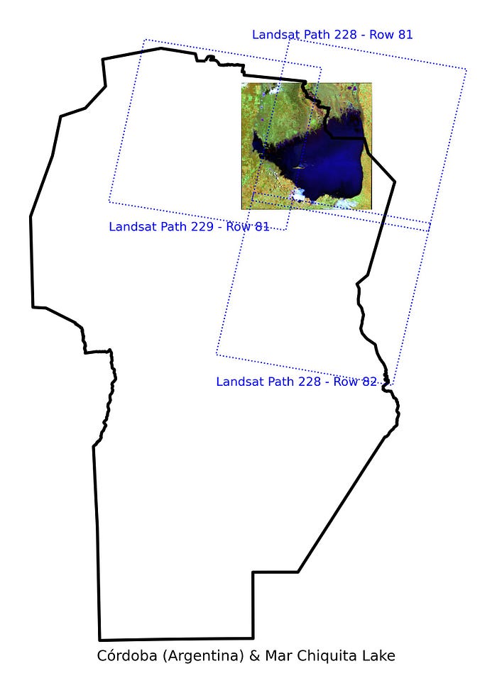
In the following image, we show a satellite image of the “Mar Chiquita” Lake, along with the “footprint” of Landsat satellites (Landsat 5 and 8) available over our region of interest (ROI). For reference, we also included a contour denoting the Córdoba province. As the image shows, we need 2 or 3 Landsat images to cover the entire ROI and assemble one Mar Chiquita image. Note that we may use just 2 patches, but this would leave us with some regions with no data. Hence, we first extract the patch that intersects our ROI from each Landsat image (identified by a Path-Row id). Then we merge all these selected patches into a single image covering the entire ROI. We will call this image the “composite.” For our particular ROI, two of the patches (228–81 and 228–82) have a time difference of a few minutes. The remaining patch (229–81) has a time difference of no greater than 7 days. For the merging process, we will assume that this time difference does not disturb the final product. From our experience, this works very well since discontinuous edges are not noticeable on the margins of the “Mar.”
Landsat data
For our study, we only considered images with an overall cloud coverage lower than 40%. The images that matched the previous criteria are:
- Landsat 5: 1986–2011 (348 images)
- Landsat 8: 2013–2021 (171 images)
That is a total of 519 images (~ 200Gb), processed without much effort thanks to rasterio, dask, geopandas, eoforge, and the ubiquitous numpy. With this set of images, we generate 168 composites (we leave 4 out of the 519 images due to quality issues).
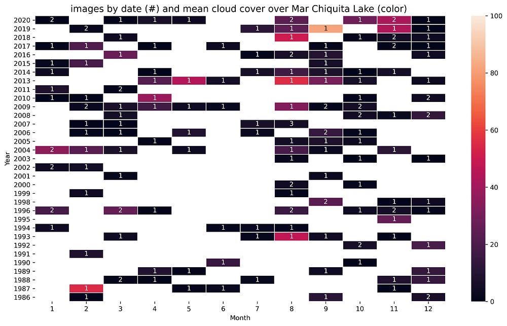

Notice that for the cloud reported in the chart above we have considered the coverage over the “Lake” only since the one informed in the metadata file refers to the whole image. That is why in some cases, you can observe some values beyond the 40% used for general filtering.
The compositing process
To construct one composite, we merge the information from 3 patches into a single image covering the entire ROI. The following figure shows 3 patches that we need to merge.
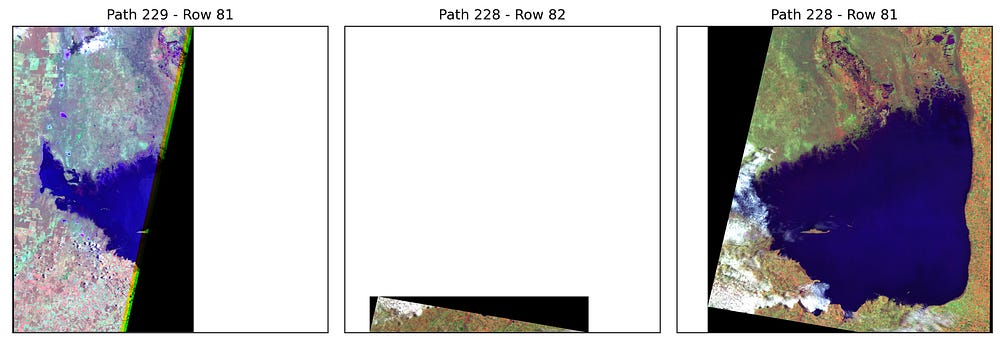
Note that the patches overlap in some regions. Therefore, we need to define how the information on the patches is used for the compositing process.
For this case study, we followed a simple compositing approach that minimizes the cloud disturbances:
- Compute the cloud mask for each patch
- Sort the patches based on their cloud cover in ascending order.
- Create an “empty composite” covering the ROI that is filled with missing data.
- Add the data from the first patch into the composite. Cloudless regions are “frozen” and cannot be modified anymore.
- Add the data from the second patch into the composite, filling regions with missing data and, if possible, replace cloudy regions with cloudless data.
- Repeat the last step for the third patch.
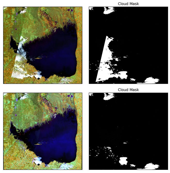
If we do not follow the compositing approach described, we may end with some “extra-cloudy” composited images. For instance, if we choose to merge the patches in the 228–81 / 229–81 / 228–82 order, we get the first pair of the upper images (bands in false color — cloud mask) and maintain most of the clouds. But, if we pick the order: 229–81 / 228–81 / 228–82, we get the two lower images, quality is good, keeping only a small fraction of clouds. In this way, we “maximize” the valid area while minimizing the cloud disturbances.
Compute the water content
After all the patches have been merged into a single composite image, we measure the area covered with water (the lake) using the Modified Normalized Difference Water Index (MNDWI). This index utilizes the green and the Middle infrared (MIR) band to detect water features, computed as:
MNDWI=(green -MIR)/(green+MIR),
whereas
NDWI = (green-NIR)/(green+NIR).
Note that this index is closely related to the normalized difference water index (NDWI) of McFeeters (1996) that uses the Near Infrared (NIR) band instead of the MIR.
Once calculated the index, we extract the Lake “mask” using simple thresholding and its corresponding polygon. Then, we may use the polygon to calculate the area, perimeter, and other geometrical properties.
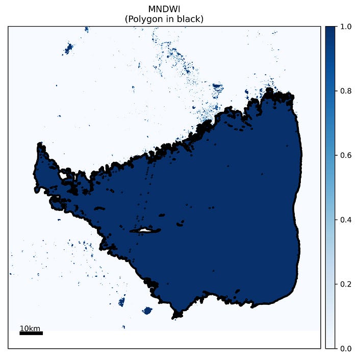
The above procedure is applied to all the composite images for the 1986–2020 period to obtain the time evolution of the Mar Chiquita area.

We observe that the area remains stable (despite the seasonal variations) in the 1986–2008 period. But from 2008 to 2013, it started to decrease (we added an — arbitrary — red dotted line at 5000 km², for reference). However, in the last five years, the lake regained a fraction of the extension lost in the previous two decades, having an extension between 3000 km² and 5000 km².
Next, we show an animation of the time evolution of the lake area. For reference, we also show, its maximum value over the the period analyzed (grey contours)
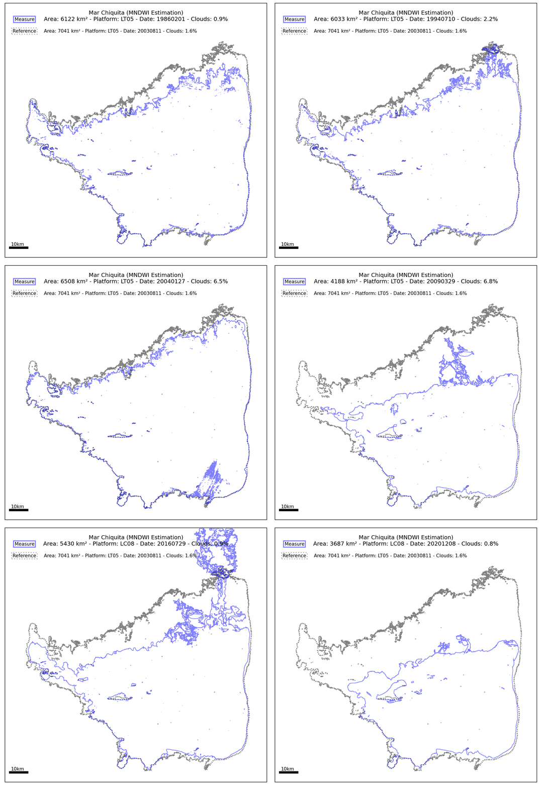
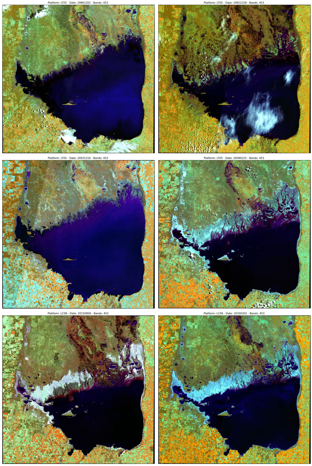
Notice that the extracted shape is not always “clean” since some artifacts like small clouds can be observed, but it gives a clear trend on Mar Chiquita area’s behavior over time. Next, we also show an animation with selected “color images’’ (False Color in this case) from Mar Chiquita. The animation shows that in some cases, the merging is smooth (we do not observe stripes along the merging border). However, in some cases we observe abrupt spatial changes in color and contrast. In future work, we will explore how this difference can be minimized by adjusting or calibrating the patches.
Final Remarks
This short article shows how remote sensing imagery can be used to monitor the spatial extent of a large water body, the Mar Chiquita lake. However, we also pointed out some of the difficulties inherent to these optical images to deal with cloudy regions. An interesting approach that we would like to explore in the future is complementing this analysis with remote sensing information from Synthetic Aperture Radars (SAR). For example, notice the benefits of (also) using SAR, Landsat8 (optical) on one side and Sentinel 1 (SAR) on the other (images from sentinel_hub):

Just one day of difference in both images, but clouds turn unusable the Landsat image (or every other optical platform with that cloud day level).
All the processing was done by using Open Source Software, using python and geo-spatial data management libraries. I hope you liked it!
I want to thanks to aperez for useful comments in the early version of this article.
